ParaFormer in production: Serving hundreds of millions of daily transformer forecasts for small business underwriting

The same attention mechanism powering frontier large language models such as ChatGPT and Claude is structurally suited to small business underwriting. A companion post “ParaFormer: A transformer architecture for small business credit underwriting“ details the model itself: how attention recovers annual seasonality from raw monthly inputs, how static features modulate the temporal pathway, and the training paradigm. This post documents the production pipeline, the modeling and engineering decisions that hold forecast robustness fixed while driving the system inside a tractable compute and latency budget.

These forecasts power real-time money movement and therefore lending at scale. At Parafin, the forecast is a critical input to offer sizing across an embedded-lending network spanning Amazon, DoorDash, Walmart, and dozens of other platforms; a tail error is not a metric regression but a missized loan. Throughput is equally consequential. Daily inference runs over years of history for more than a million merchants, ingesting billions of input points and emitting 17 quantiles across a 12-month horizon per merchant. Hundreds of millions of predictions per day. The objective is to preserve forecast robustness under a fixed compute and latency ceiling.

The remainder of this post describes how we met both targets: forecast robustness that improves on the prior production system, with daily inference completing in under an hour at population scale.

1. Population segmentation and temporal granularity

The first lever is scope. Not every merchant warrants a deep sequence model, and not every temporal resolution justifies its compute. Fixing these boundaries early maximizes both robustness and efficiency.

1.1 Routing by data density

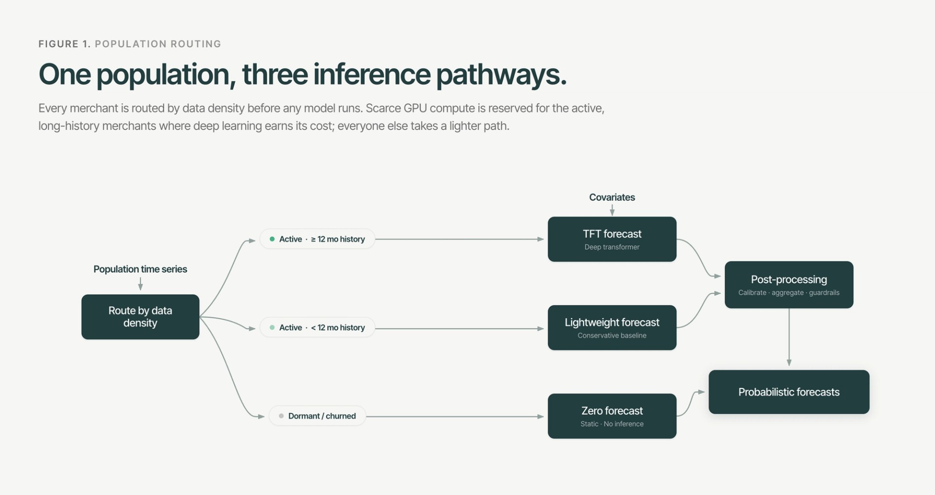
We partition the 1M+ merchant population into three inference pathways:

• Dormant and churned accounts — zero sales over the trailing 12 months bypass model inference entirely and receive a static zero forecast.
• Active, short-history merchants (<12 months) route to a lightweight, conservative model. The TFT’s self-attention is engineered to capture long-range temporal dependence and annual seasonality; on sub-annual sequences it confers no advantage.
• Active, long-history merchants (≥12 months) pass to the full TFT pipeline.

This routing avoids over-fitting forecasts to sparse data. The lightweight model is a low-variance safety net for newer merchants; scarce GPU compute is reserved for the active long-history population, where deep learning delivers material accuracy gains.

1.2 Monthly granularity as a noise filter and a compute lever

The system operates entirely at monthly resolution. Against a 32-month context window and a 12-month prediction horizon, monthly granularity compresses encoder and decoder sequence length roughly 30× relative to daily data, directly relaxing the quadratic memory and FLOP cost of attention. Aggregation doubles as a signal-processing filter: it removes high-frequency structure, weekend cycles, single-day anomalies and payout-day clustering that is irrelevant to advances underwritten over 3-to-12-month terms, raising the signal-to-noise ratio of the long-horizon seasonal trends the TFT is built to capture.

2. Post-inference calibration and joint aggregation

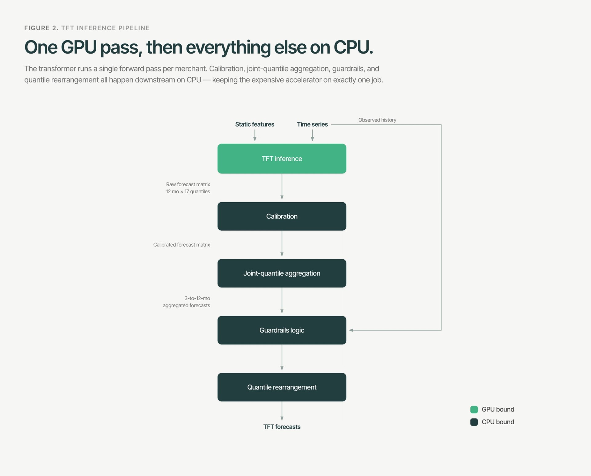
The model emits per-month marginal quantiles in a single forward pass. Two properties the downstream underwriter requires, empirical calibration and a coherent multi-month joint distribution, are not guaranteed by the training objective alone. We recover both in a two-stage CPU pipeline, leaving the GPU to execute exactly one forward pass per merchant.

Concretely, the TFT emits marginal quantile predictions per (series, future month) in a single forward pass via QuantileOutput, producing a 17-point grid over α ∈ {0.10, 0.15, …, 0.90}. Converting these raw marginals into the calibrated, joint-quantile predictions the underwriter consumes proceeds in two stages, executed entirely on CPU.

2.1 Multiplicative marginal calibration

The pinball loss is a proper scoring rule for quantile estimation, but minimizing it does not enforce empirical calibration out of sample: the raw predicted quantile ŷα can deviate from the true α-quantile of the conditional distribution. We correct this post hoc with a per-quantile multiplicative factor cα, fitted as the α-quantile of the historical forecast ratios y/ŷα. Scaling the raw prediction by cα aligns the outputs with empirical targets. For statistical robustness, each factor is fitted on a minimum of 103 observations, clipped, and shrunk toward 1.0 by a regularization hyperparameter.

2.2 Joint-quantile horizon aggregation via Gaussian copula

Capital advances are sized against cumulative sales over a multi-month horizon:

S = Σh=1H Yh.

The naive marginal-sum identity

qα(S) ≈ Σh=1H qα(Yh)

holds exactly only under strict co-monotone dependence. In practice this assumption mis-calibrates: below the median (α < 0.5) the right-hand side is sub-additive and overly pessimistic; above the median (α > 0.5) it is super-additive and overly optimistic. The failure mode is concrete under naive marginal-sum aggregation, observed coverage at q0.10 falls materially below its nominal 10% target over long horizons.

Recovering the true joint distribution natively, inside the network, would require sampling 12-month paths: K forward passes per batch, with K ≈ 300 for adequate precision. Across a million-plus merchants, this amounts to hundreds of millions of GPU forward passes per day.

Instead we preserve the single GPU forward pass and reconstruct the joint distribution on CPU via a Gaussian copula. Passing the predicted marginals through their CDFs and mapping to standard-normal space via the inverse normal CDF, we model the horizon as multivariate normal with covariance Σ, parameterized as an AR(1) Toeplitz matrix with a single correlation parameter ρ estimated on held-out validation data.

Relocating the joint construction to CPU unlocks Quasi-Monte Carlo integration. We draw scrambled Sobol’ sequences with antithetic pairing in standard-normal space; K1 = 128 base draws achieve precision equivalent to K2 = 103 pseudo-random draws across the H = 12 month horizon. Because the latent samples are shared globally across all series, memory scales as O(K1H) rather than O(NK2H) for N > 1M merchants, collapsing a footprint exceeding five billion scalar elements to a globally shared array of ~1,500 elements that resides in CPU cache, so the per-series inverse-CDF lookup is fully vectorized. The result captures month-over-month temporal dependence without the co-monotonicity flaw; the entire CPU stage completes in minutes, displacing the heavy GPU path-sampling an in-model approach would demand.

3. Downstream guardrails and ensembling

Deep models extrapolate poorly at the edges of their training distribution. In our case, those edges are merchants with a short history. Since the output sizes are real capital, we bound that error with three mechanisms applied in series before the forecast reaches the underwriter.

3.1 Dual-anchor guardrails

Post-aggregation quantiles are clipped to a plausible band defined by two independent, data-derived anchors per series:

• The recency anchor: the mean of the trailing six months of observed sales tracks the merchant’s current operating level.
• The periodicity anchor: the mean of the corresponding calendar months in prior years preserves expected annual seasonality.

Per (series, quantile, horizon), the upper and lower bounds are scaled by factors that respect strict quantile monotonicity, so clipping cannot itself introduce new quantile crossings and the prediction grid retains structural integrity.

3.2 Quantile rearrangement

Minor crossings can survive even monotone clipping. We eliminate them with the rearrangement operator of Chernozhukov, Fernández-Val, and Galichon (2010): sorting the multiset of clipped values per series and reassigning them to quantile labels in strictly increasing order removes all crossings while preserving the empirical distribution without systematic shift.

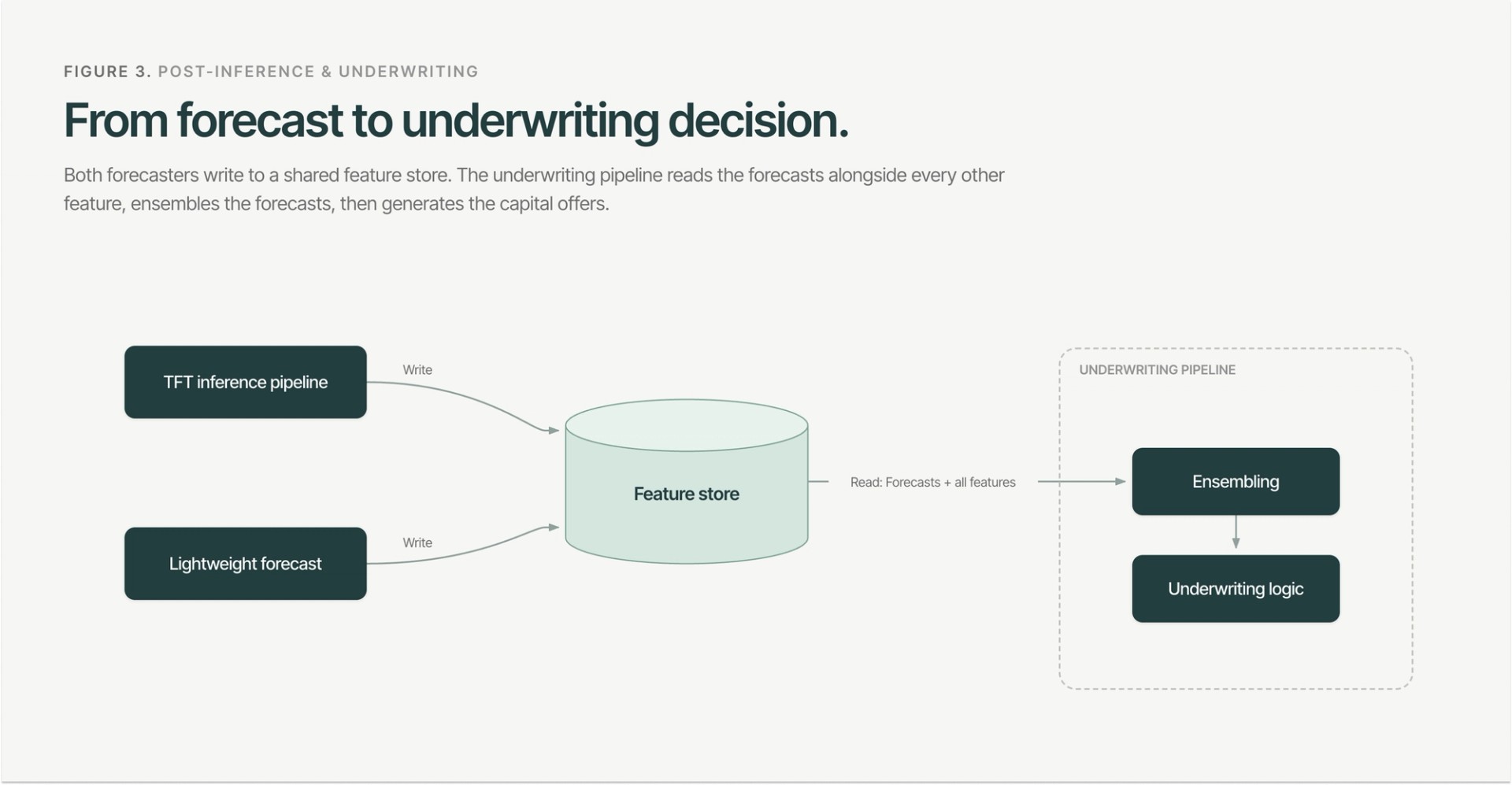
3.3 Smooth on-ramp ensembling

We blend the lightweight model and the TFT across three history tiers to avoid discontinuities in capital offers as merchants accumulate data:

• < 12 months: lightweight model only. Short sequences offer the TFT no predictive advantage while adding compute and extrapolation risk.
• 12–24 months: a convex combination of the two, weighted dynamically by context length. Because TFT accuracy rises monotonically with context, shifting weight linearly toward it tracks the model’s real performance ramp and prevents step-changes in offer sizing at the 12-month threshold.
• > 24 months: pure TFT, where its empirical advantage is largest.

4. Looking ahead: Scaling deep learning safely

Monthly granularity shrinks sequences ~30x and attention work by ~900x. Downstream, the copula-based aggregation step replaces hundreds of millions daily GPU forward passes with a lightweight CPU step, and quasi-Monte Carlo matches the precision of 1,000 random draws with just 128. Compounded, these choices serve hundreds of millions of daily forecasts in under an hour on a single A10 GPU.

Putting a transformer like ParaFormer into production means solving statistical robustness and compute efficiency simultaneously. The system above is the product of a co-designed stack in which Parafin’s data science and engineering teams optimize algorithm and infrastructure concurrently across billions of daily inputs, a million-plus merchants, sub-hour population-scale inference.

The pipeline establishes a reusable blueprint: state-of-the-art deep learning can be deployed safely, efficiently, and at population scale in a regulated credit setting. As Parafin extends its underwriting capabilities across the embedded-lending partner ecosystem, this architecture is the template for reliable, real-time capital movement. If work like this excites you, we are hiring!

References

Chernozhukov, V., Fernández-Val, I., & Galichon, A. (2010). Quantile and probability curves without crossing. Econometrica, 78(3), 1093–1125.

Lim, B., Arık, S. Ö., Loeff, N., & Pfister, T. (2019). Temporal Fusion Transformers for interpretable multi-horizon time series forecasting. arXiv:1912.09363.